Locals observe large differences in precipitation on short distances, and people have done for generations. They witness the terrain’s large influence on rain, especially in mountainous areas. Here in western Norway the air is often very moist when it approaches the mountains. Ahead of the mountain base the air is forced upwards. As the air rises it cools and some of the water condenses, leading to a larger amount of droplets. These are too heavy to stay in the air, and tend to fall towards the ground the day you have outdoor plans. On the other side of the mountain however, the air sinks and can again contain larger amounts of water in vapour form. The droplets evaporate, and it stops raining. We know that even small hills can influence where the precipitation falls, but the official observation network is too sparse to catch these very local variations. Therefore, as an addition, we use numerical models to estimate precipitation distribution.
A numerical model is a picture of the world in squares. Models that include the entire globe usually have square sizes of roughly 100 km x 100 km. This put, for example, Bergen and Voss in the same square, which implies that they have the same climate. This is definitely not the case. Therefore, when we wish to study small scale phenomena, as terrain induced precipitation often is, we need considerably smaller squares. The model calculations take much longer time as there are many more squares, but the end result opens up for many more details.
The advantage of having many, smaller squares is that the complex terrain we see outside the window is now more realistically represented in the model. Before there was one square with one altitude at the Bergen-Voss point. Now that square is divided into 100 x 100 squares with 10.000 different altitudes. As seen in Figure 1 the terrain in the model becomes more detailed with increased amounts of squares, we can see deep valleys and the high mountains, which forces the air to rise. And remember, this is one of the factors we know is important for precipitation distribution. With one square the precipitation is the same in the whole square. With many squares, we open up for the local differences. One should think that the more, smaller squares the better, but is it always so?
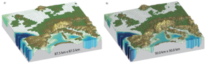
Figure 1: The square sizes vary and the terrain is differently represented in the models. The smaller the squares the more details the terrain has. Source: IPPC.
We have investigated just that, and found that smaller squares are not always better (Pontoppidan et al. 2017). We studied a heavy precipitation event in western Norway, and found that adjusting square size from 9 km to 3 km improves the model considerably. The 3 km squares gave much more realistic rainfall, but when we reduced to 1 km squares this did not improve much. Why? We believe this is related to how the weather model represents the terrain. In Figure 2 the terrain, shown in grey, is clearly less detailed in the 9 km simulation than in the remaining two. The 1 km terrain however has to be smoothed (so the weather model does not crash), but is still more detailed than with 3 km squares. The red and blue colours in the figure show the vertical movement of the air (remember rising air causes rain) and we see that air moves up and down in a wave pattern over the mountains, at least in the 3 km and 1 km simulations. The terrain-forced wave motion can enhance precipitation, leading to large local differences similar to what inhabitants have observed. Our experiments show that the square size matters. However, if we want to simulate the weather that locals observe in mountain areas, it is as important that our models include the detailed terrain. When it comes to square sizes in numerical models, smaller is not always better.
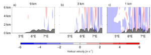
Figure 2: The model simulation of air forced above the terrain, here shown as vertical velocity of the air. Three different square sizes are shown (9 km, 3 km and 1 km).
Citation:
Pontoppidan, M., Reuder, J., Mayer, S., & Kolstad, E. W. (2017). Downscaling an intense precipitation event in complex terrain : the importance of high grid resolution. Tellus A. Early online release. http://www.tandfonline.com/doi/full/10.1080/16000870.2016.1271561
 0
0
 0
0 0
0 0
0 0
0 0
0Marie Pontoppidan
Latest posts by Marie Pontoppidan (see all)
- Terrain and climate models - April 24, 2017