When modelling the natural world we are often faced with limitations of our understanding, available computing resources, or model grid resolution, and need to simplify the equations – parameterize a process. While such parameterizations are often useful, making near-impossible possible, there are certain caveats which one might not think about that often.
First, when we parameterize a process which we do not completely understand, we introduce it through a simplified relation. We use observations to look for simple empirical (observed) relationships between constant or variables that we can model and the variables that we want to describe. In a similar way we often simplify the equations when we are dealing with very complicated systems that would take too much time to calculate when fully described. Simple equations are often easy to understand and very useful in simple settings, but can produce wrong results in more complicated environment. Therefore one needs to take special care when a parametrization is used for the first time in a new setting.
Second, we parameterize processes which are so small that they cannot be solved in a model grid. The model equations can often reproduce these processes, but the model simply doesn’t see them, which is why they have to be incorporated to models in some other way. An example of such process are the meso-scale eddies, the “ocean weather”, which are important for transport and mixing1 of properties such as momentum, heat, and salt among others. These eddies are problematic since models’ ability to reproduce them is scale dependent. While models with large grid size (~100 km) will perform poorly without a parameterization, a model with small enough grid size (<10 km) will reproduce the eddies making the parametrization obsolete (See Figure 1 and a nice simulation of the problem by GFDL).
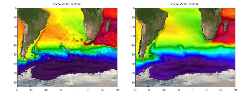
Simulations with Norwegian Earth System model showing sea surface height at two resolutions: at 1/4° (~25 km) without an eddy parameterization on the left and at 1° (~100 km) on right with an eddy parameterization. Note how the large scale patterns are similar, but the 1/4° simulation starts to show eddy structure, especially the Agulhas leakage is much more pronounced showing several Agulhas rings. Figures are courtesy of Dr. Mehmet Ilicak
Most of the current climate models are in a gray zone where they reproduce some of the larger eddies, but not the smallest ones (so called eddy-permitting model resolution). This is obviously problematic; turning the parametrization on while already solving some eddies could result in too large mixing, but on the other hand the mixing due to missing eddies should be parameterized. On the other hand the parameterizations also tend to smooth the horizontal temperature and salinity contrasts, which are the fuel for the eddies in the first place, leading to less eddy activity than the model could reproduce. A further complication is that the size of the eddies depends on the latitude and vertical ocean stratification, largest eddies occurring generally closer to the equator2 and in weakly stratified waters. In the gray zone of eddy-permitting model resolution we often gradually turn down the parameterization in areas where the model starts to solve the eddies.
Finally, parameterizations are usually ‘calibrated’ with the current climate, their constants are tuned to match the observations, which is why the largest uncertainties arise when we simulate extreme future or past climates. Simply because the relationships are true in the current climate does not mean that they would hold in much different conditions. A simple parameterization is useful here as well – it is often easier to know when the results are unreasonable, and especially why. While parameterizations are simplifications by definition, and thus not perfect, the best ones are easy to understand and allow us to include many processes into the models and still solve the equations in a reasonable time.
Footnotes
1 Mixing in general is a good example of the type of process that needs to be parameterized. In fact, the scales of mixing go down all the way to the molecular scales where the kinetic energy is dissipated, and there is no climate model which would reproduce mixing across all the scales. So in the end some mixing will always be parameterized.
2 This is because the Rossby radius depends on the latitude
Some sources and extra reading on eddies and parameterizations
Mesoscale eddies at GFDL website
Isaac Held on eddy resolving models
Fox-Kemper et al., on submesoscale process
 0
0
 0
0 0
0 0
0 0
0 0
0Aleksi Nummelin
Latest posts by Aleksi Nummelin (see all)
- Simplifying the equations - February 11, 2016
- Small talk – the model way - May 17, 2013
- Norway and the USA: two countries, two cultures – one science? - March 29, 2013