Scisnack | Polar lows: what fuels Arctic hurricanes?

What are polar lows?

Through the centuries seafarers in the Nordic Seas have told tales of unexpected encounters with severe storms that appeared out of nowhere to wreak heavy snowfall, fierce wind and huge waves on their ships. With the advent of satellites, it was noticed that these unpredictable low-pressure vortices are ubiquitous over high-latitude seas, and a name polar low was proposed. You may hear of them as comma clouds, explosive mesocyclones, Arctic instability lows, Antarctic coastal vortices and, when having a clear eye in the centre – Arctic hurricanes [1].

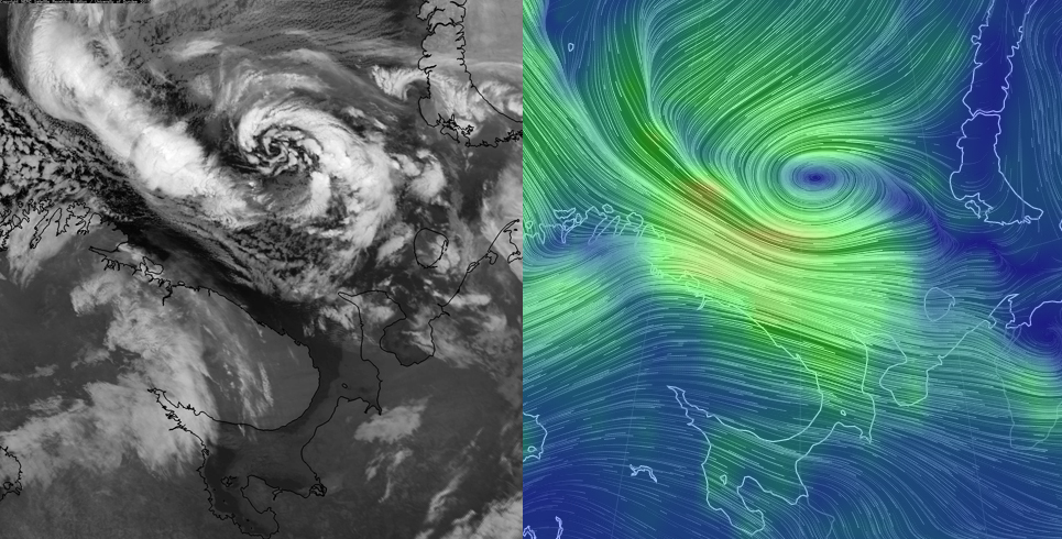
Figure 1: (Left) Polar low over the Barents Sea. 13 February 2015. NOAA satellite image. Source: NERC Satellite Receiving Station, Dundee University, Scotland. (Right) Polar low over the Barents Sea. 13 February 2015. Visualisation of surface wind in Global Forecast System. Reddish colors indicate wind speeds reaching 25 m/s. Source: Earth, a visualisation of global weather conditions.

Being the most dangerous member of the polar mesoscale cyclone family, polar lows are usually characterized as small (100–500 km in diameter) and short-lived maritime depressions with near-surface winds exceeding 15 m/s (Figure 1). Even nowadays severe weather associated with polar lows and the difficulty in producing accurate forecasts of their occurrence continues to make them a hazard to ships, oil rigs and coastal communities in the Arctic, North Atlantic and North Pacific.

In January 2003, a strong polar low coursed as far south as to hit the British Isles, causing severe blizzards over much of the UK as well as over large parts of the Netherlands and Belgium. At some locations on the eastern shores of England wind speeds reached 25-28 m/s. That afternoon chaos reigned throughout Great Britain. Stansted Airport was closed, flights were cancelled at Heathrow Airport, the London underground came to a halt, schools were closed, many workers found themselves in traffic gridlock for many hours, thousands suffered power cuts, and there were numerous road accidents as up to 15 cm of snow fell in many places. Yet in the corresponding satellite image the following day, only a tenuous streamer, possibly a remnant of the cyclone’s ‘comma’ tail, remained to tell the tale [2].

This example shows how violent and disruptive these polar storms can be, even when they are in the decaying stage over the land. And if this vivid picture does not impress you, maybe the amount of energy released by a polar low would be more convincing.

How energetic are polar lows?

From school we know that an object’s kinetic energy is proportional to mass and velocity squared. For an atmospheric vortex these quantities can be expressed in mass of a unit air column, convective flux and the Coriolis parameter [3]. Typical conditions observed inside a polar low give an estimate of roughly 10¹⁸ J of the total kinetic energy. It is indeed an enormous amount of energy! Taking into account its short lifetime, it turns out that a polar low is 50 times more powerful than the total average electricity consumption in the counties within the ClimateSnack community [4]. Compared to atmospheric phenomena, polar lows are generally less powerful than a mature tropical cyclone (which possesses roughly 10¹⁹ J of energy per day), but hundreds of times more energetic than a single thunderstorm [5].

But how on Earth do these polar lows become so powerful? Research findings offer several answers to this question. Due to the fact that polar lows develop in high-latitudes over the sea surface, their energy cycle is based on dynamics of both tropical hurricanes and mid-latitude cyclones.

Similarities with mid-latitude cyclones

A feature that many polar lows have in common with synoptic-scale mid-latitude cyclones is known as baroclinic instability. This scary term stands for a process that can occur in the baroclinic atmosphere – in which air density depends on both the temperature and the pressure [6]. The Earth’s atmosphere is almost always baroclinic, rather than barotropic (when air density depends only on the pressure). In the baroclinic atmosphere on a surface of constant pressure, the temperature varies – a temperature (and hence density) gradient exists. A simple example is two adjacent air masses: a warm and a cold one.

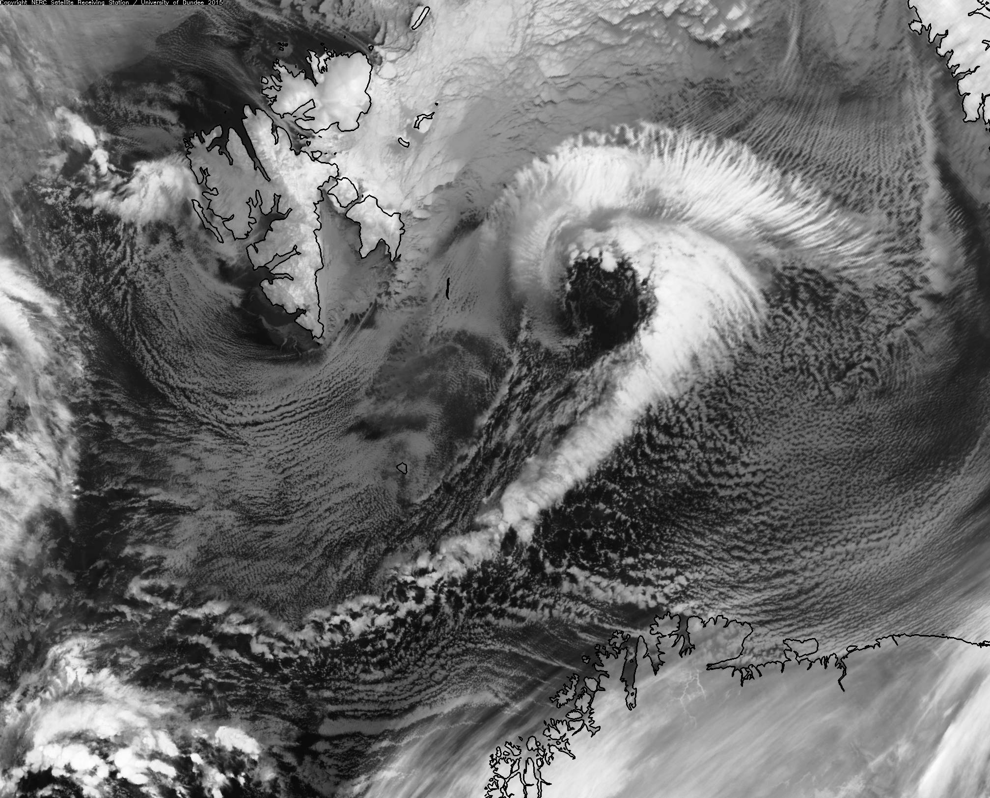
NOAA satellite image of comma-cloud polar low over the Barents Sea east of the Svalbard Archipelago. 1 February 2015. Source: NERC Satellite Receiving Station, Dundee University, Scotland.

Figure 2: NOAA satellite image of comma-cloud polar low over the Barents Sea east of the Svalbard Archipelago. 1 February 2015. Source: NERC Satellite Receiving Station, Dundee University, Scotland.

The temperature gradient is proportional to the so-called available potential energy (APE). As you might guess, like any object in the planet’s gravitational field, the atmosphere has potential energy. A part of potential energy can be converted to the energy of atmospheric motion; hence, it is called available. The essential part of the conversion is vertical movement of air – this is how the air masses approach equilibrium, consuming APE. APE is actually a tiny bit of the total amount of energy (about 0.5%), but in the absence of other energy sources it is the only reservoir that can feed the atmospheric circulation.

Strong temperature gradients are common in the polar atmosphere, for example, during massive outbreaks of cold air over warm ocean surface. As a result, sharp baroclinic zones develop, and a vortex can grow bigger and bigger, drawing energy from the APE of the mean flow.

It is believed that APE is one of the primary energy sources for polar lows. It prevails over other sources, especially when a polar low appears as a comma-shaped cloud on the satellite images (Figure 2).

Similarities with tropical cyclones

When you first saw the satellite images in this post, I bet you immediately thought of tropical hurricanes. This is not surprising, as many polar lows look like small tropical cyclones straying too far from their warm home (Figure 1, 3). But could a polar low really develop in the same way as its tropical cousins do – and brew up on the ocean’s heat?

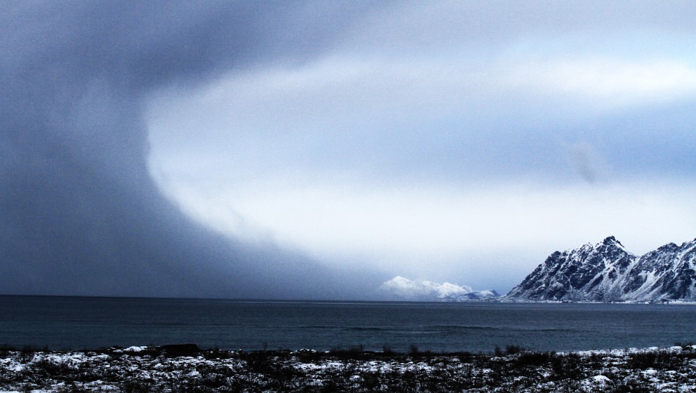
Figure 3: Polar low approaching Lofoten islands. 19 December 2014. Source: NRK.no

The idea of air-sea interaction (Figure 4a) has been successfully applied to tropical cyclones and has gained popularity in polar lows studies. It postulates that wind-induced heat exchange near the sea surface plays the key role in cyclone growth. The process is essentially the same as when you blow on a cup of tea, heat is transferred to the air, and tea cools down. More precisely, induced by strong surface winds, excessive heat comes from the sea surface and increases temperature anomalies inside a cyclone. This, in turn, further strengthens the area of low pressure and therefore enhances surface winds. A positive feedback is established.

Another way of hurricane intensification also relies on heat released from the ocean. But instead of wind-driven turbulent transfer of energy from the surface, it requires the convergence of moist air in the centre and the presence of convective energy stored in the atmosphere (Figure 4b). The release of that energy occurs when water vapour contained in the lifted air condenses and forms spectacular cumulonimbus clouds. So as you might know, this mechanism resembles the formation of a regular thunderstorm.

Recently, more scrupulous observations have shown that the Arctic atmosphere does not favour the accumulation of the required amount of convective energy for long enough. Thus, condensational heating on its own does not represent a significant part of the energy budget of the majority of polar lows [7]. However, acting along with baroclinic processes (see the previous section) it can boost the rapid development of a polar low.

In the real world the two mechanisms described here are usually hard to distinguish. More importantly, both of them require a pre-existing trigger to kick an engine of a polar low. Can an island or maybe a sea-ice edge act as a trigger? Quite possibly, but each polar low story is unique.

Figure 4: How surface heat fluxes fuel polar lows (a).
How condensational heating fuels polar lows (b). Adapted from [8].

A few words about shear lines

All three mechanisms that we have already looked at attribute generation of kinetic energy to conversion from the potential energy. The difference was only in a way by which the potential energy was created and released.

But polar lows over regions like the Labrador Sea or the Japan Sea, can be of different origin, namely barotropic. Their primary energy source is large-scale kinetic energy. What is a recipe for barotropic polar low? Firstly, you need a large-scale flow with high speed and thus large amounts of kinetic energy. And secondly, a strong enough wind shear must be present. The shear line will give birth to waves and whirls of various sizes. It means that the large-scale flow transfers kinetic energy to smaller scale vortices, the largest of which then can become a polar low [8].

Blending dynamics together

OK, now that we have learned some physics involved in polar low development. Can we apply theory into practice? Well, yes, but it’s far from being straight-forward. Polar lows rarely feed exclusively on one energy source; almost always there is an interaction between sources during the sea adventures of a polar low. For instance, studies indicate that initially barotropic vortices forming along a shear line may cause intense convection within a limited region and trigger a convectively driven polar low [8].

The best way to understand such a complex phenomenon is to make maximum use of observations. Currently, my humble contribution to this research area is aircraft data analysis of the polar low, which developed during a strong cold-air outbreak near Svalbard. But there is a great demand for further targeted observations of these weather systems, which will help to improve short-range weather forecasts and thus reduce economic losses by correctly planning our activity in polar seas.

Summary

Polar lows are small and ferocious maritime cyclones, characterized by the total amount of kinetic energy reaching 10¹⁸ J.
Their chief energy sources are: air-sea heat fluxes, condensational heating; available potential and kinetic energy of large-scale flow.
Almost always a polar low lives by a complex and non-linear interactions between energy sources. The question is what is the relative importance of each of them in a particular polar low and whether a new unifying concept of polar low can be developed.
If you got fascinated by the beauty and complexity of polar low phenomenon, I highly recommend reading a very nice blog about polar lows, with self-explanatory title: “the coolest weather on Earth”.

References

[1] Renfrew IA. 2003. Polar lows. In Encyclopedia of Atmospheric Sciences (pp.1761–1768). Elsevier.

[2] Hamilton L. 2003. The polar low phenomenon. GEO Quaterly, (1).

[3] Golitsyn GS. 2008. Polar lows and tropical hurricanes: Their energy and sizes and a quantitative criterion for their generation. Izvestiya, Atmospheric and Oceanic Physics, 44(5):537–547.

[4] CIA World Factbook, Electricity – Consumption. https://www.cia.gov/library/publications/the-world-factbook/rankorder/2233rank.html.

[5] Wikipedia, Orders of magnitude (energy). http://en.wikipedia.org/wiki/Orders_of_magnitude_(energy).

[6] Holton JR. 2004. An Introduction to Dynamic Meteorology. International Geophysics. Elsevier Science.

[7] Linders T and Saetra Ø. 2010. Can CAPE Maintain Polar Lows? Journal of the Atmospheric Sciences, 67(8):2559–2571.

[8] Rasmussen EA, Turner J. 2003. Polar lows: mesoscale weather systems in the polar regions. Cambridge University Press: Cambridge, UK.